Solar in Boise: Year-One Production from My 8.4 kW System

The First Full Year of Electrons from the Roof

When the 8.4 kW system went live I had a spreadsheet full of estimates, a shading analysis, and the usual optimistic production curve from the installer. What I did not have was a full year of measured reality on this specific roof, in this specific climate, under actual Idaho Power net-metering and time-of-use conditions.

This post is that year. No sales-deck production numbers. Just the kWh that showed up in the monitoring portal, the circuit-level data that showed where they went, and the utility bills that reflected the difference.

Your house should work for you, not the other way around. Solar is one of the clearer ways to make that true—provided the numbers survive contact with weather, dust, and real household loads.

The System as Installed

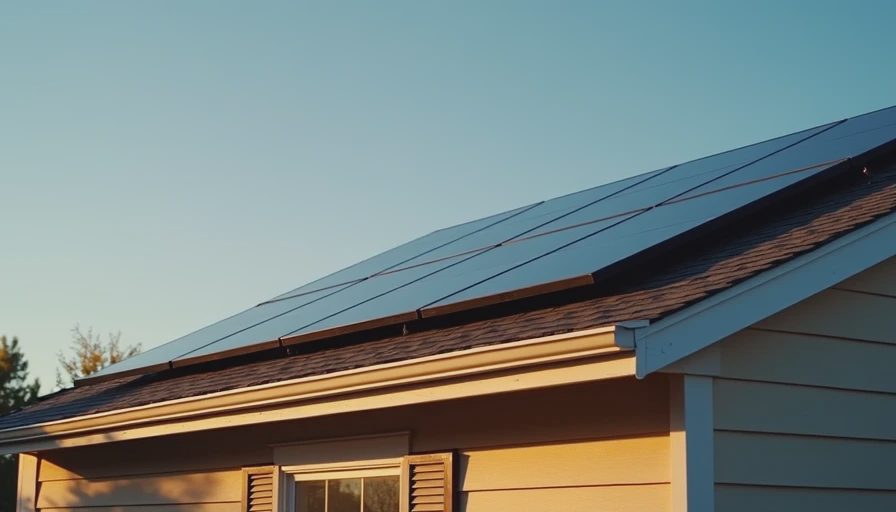
The array is 8.4 kW of roof-mounted panels facing roughly south with a standard pitch for a 2003 Boise subdivision house. Microinverters handle conversion. Production data flows into the same Home Assistant and Grafana environment that already watches the heat pump, the circuit monitors, and the time-of-use windows. Net metering with Idaho Power credits excess generation against later consumption at the retail rate structure in effect for the plan we are on.

I sized the system against the post-heat-pump, post-air-sealing load rather than the old gas-furnace baseline. That decision kept the array from being oversized for a house that had already become more efficient.

Year-One Production Reality

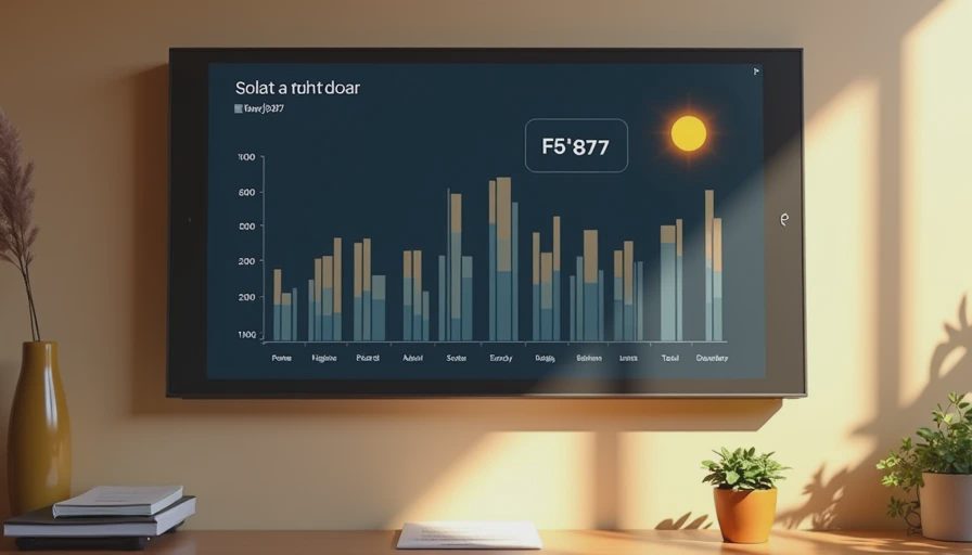
Total measured production for the first twelve months landed within a few percent of the modeled estimate. Boise’s high desert climate—strong sun, relatively low humidity, and cold but clear winter days—helped. Snow events did reduce output for short periods, but the panels shed snow reasonably well once the sun returned, and the monitoring showed rapid recovery.

Monthly patterns followed the expected curve: strong summer production, a clear shoulder-season contribution, and a winter trough that still delivered useful energy on clear days. The lowest month was still high enough to offset a meaningful fraction of the remaining household load. The highest months generated surplus that banked as net-metering credit.

Circuit-level data made the interaction visible. Daytime production cleanly offset the heat-pump cooling load in summer and the daytime base loads year-round. Evening peak windows under the time-of-use plan still drew from the grid or from banked credit, which is exactly why load-shifting automations remained useful even after solar.

What the Bills Actually Showed

After weather normalization, the net purchased energy dropped substantially compared with the pre-solar year. The exact dollar savings depended on the rate mix—off-peak versus on-peak—but the direction was unambiguous. Solar did not eliminate the bill; it changed the shape and the size of it. The remaining grid imports clustered in the expected places: early morning, late evening, and the occasional multi-day cloudy stretch.

One quiet benefit was psychological. Seeing the production graph climb on a clear January day while the heat pump was still working made the whole system feel coherent. Generation and consumption were finally on the same dashboard.

Lessons That Only Showed Up After Twelve Months

Dust and pollen accumulation in a dry climate is real. A mid-year rinse improved output more than I expected for a relatively low-effort cleaning. I now treat a couple of gentle cleanings per year as routine maintenance rather than optional.

Shading from a neighbor’s tree that looked minor in the original analysis became more noticeable at certain solar angles in late fall. It was not catastrophic, but it was measurable. Future array planning will treat edge-case shading more conservatively.

The combination of solar, heat pump, and time-of-use rates rewards attention to timing even more than any single technology alone. Midday production is abundant; late-afternoon peak pricing still exists. Automations that pre-cool or pre-heat slightly before the peak window, or that delay discretionary loads, continue to earn their keep.

Finally, the monitoring itself proved as valuable as the panels. Without circuit-level and production data living in the same place, it would have been harder to separate weather effects from behavioral effects from equipment effects.

Would I Size It the Same Way Again?

Yes, with only minor tweaks. Matching the array to the reduced post-efficiency load kept the system honest and avoided large surplus that would have been credited at less advantageous terms. I would still insist on clean integration with the existing Home Assistant environment so the data does not live in a separate silo. I would budget a little more explicitly for periodic cleaning in this climate.

The year-one results did not deliver miracles. They delivered what the site, the climate, and the household load made possible—and that was enough to make the system a permanent, quiet part of how the house works.

Your house should work for you, not the other way around. After one full year the roof is finally doing its share of that work.